google实时土地覆盖数据

简介

数据名称：Dynamic World NRT

数据范围：全球

数据时效：2015年6月23日-至今

数据说明：全球土地覆盖产品历来每年生产一次，在图像处理和数据集发布之间往往有很大的滞后时间。Google开发了一种新的自动化方法，利用对 10 mSentinel-2 影像的深度学习，实现全球一致的高分辨率近实时 （NRT） 土地利用土地覆被 （LULC） 分类，包含9个土地覆被类型：水体、草地、森林、淹没植被、农田、灌木、建设用地、裸地、冰/雪。

数据生产流程

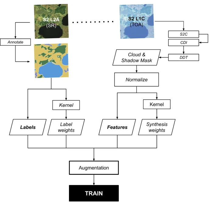
模型是使用手工注释图像和无监督方法的组合进行训练的，用于使用地球引擎和Google Cloud AI平台上的云计算，为新的和历史的Sentinel-2图像生成LULC类概率的NRT预测。Dynamic World 为用户提供了更大程度的灵活性，以生成根据其需求和研究领域量身定制的自定义聚合和衍生产品。Dynamic World NRT产品从2015-06-27至今可用于完整的Sentinel-2 L1C系列。根据纬度的不同，Sentinel-2 的重访频率在 2-5 天之间。

精度对比

Dataset	NRT	Global	Agreement	Scale (m)	Tiles
Mapbiomas Amazonia 2018 (N.Brazil, Venezuela, Peru, Bolivia)	No	No	54.8%	30	11
ESA S2GLC Europe 2019	No	No	59.2%	10	45
ESA CCI 2018	No	Yes	61.6%	300	409
ESA CGLS ProbaV 2019	No	Yes	66.3%	100	409
NLCD 2016 (30 m, CONUS + Alaska)	No	No	66.7%	30	56
Mapbiomas Brazil 2019	No	No	67.4%	30	20
LCMAP 2017 (30 m, CONUS only)	No	No	75.0%	30	48
Dynamic World (NRT)	Yes	Yes	73.8%	10	409

（与其他同类数据产品精度对比）

土地覆盖分类

Dynamic World 土地覆被分类表

Class ID	LULC Type	Description	Examples
0	Water	• Water is present in the image. • Contains little-to-no sparse vegetation, no rock outcrop, and no built-up features like docks. • Does not include land that can or has previously been covered by water.	• Rivers • Ponds & Lakes • Ocean • Flooded Salt Pans
1	Trees	• Any significant clustering of dense vegetation, typically with a closed or dense canopy. • Taller and darker than surrounding vegetation (if surrounded by other vegetation).	• Wooded vegetation • Dense green shrubs • Cluster of dense, tall vegetation within savannas • Plantations such as apples, bananas, citrus, and rubber • Swamp (dense/tall vegetation with no obvious water) • Any mix of the above • Any burned areas of the above
2	Grass	• Open areas covered in homogenous grasses with little to no taller vegetation. • Other homogenous areas of grass-like vegetation (blade-type leaves) that appear different from trees and shrubland. • Wild cereals and grasses with no obvious human plotting (i.e. not a structured field).	• Natural meadows and fields with sparse or no tree cover • Open savanna with little to no tree cover • Parks, golf courses, human manicured lawns, including large fields in urban settings like soccer and baseball. • Tree cut-throughs for power lines, gas etc. • Pastures • Reeds and marshes with no obvious flooding
3	Flooded vegetation	• Areas of any type of vegetation with obvious intermixing of water. • Do not assume an area is flooded if flooding is observed in another image. • Seasonally flooded areas that are a mix of grass/shrub/trees/bare ground.	• Flooded mangroves • Emergent vegetation
4	Crops	• Human planted/plotted cereals, grasses, and crops.	• Corn, wheat, soy, etc. • Hay and fallow plots of structured land
5	Shrub & Scrub	• Mix of small clusters of plants or individual plants dispersed on a landscape that shows exposed soil and rock. • Scrub-filled clearings within dense forests that are clearly not taller than trees. Appear grayer/browner due to less dense leaf cover.	• Moderate to sparse cover of bushes, shrubs, and tufts of grass • Savannas with very sparse grasses, trees, or other plants
6	Built area	• Clusters of human-made structures or individual very large human-made structures. • Contained industrial, commercial, and private building, and the associated parking lots. • A mixture of residential buildings, streets, lawns, trees, isolated residential structures or buildings surrounded by vegetative land covers. • Major road and rail networks outside of the predominant residential areas. • Large homogeneous impervious surfaces, including parking structures, large office buildings, and residential housing developments containing clusters of cul-de-sacs.	• Cluster of houses, can include smalls lawns or small patches of trees can be included • Dense villages, town, and cityscape (buildings and roads together) • Clusters of paved roads and large highways • Asphalt and other human-made surfaces
7	Bare ground	• Areas of rock or soil containing very sparse to no vegetation. • Large areas of sand and deserts with no to little vegetation. • Large individual or dense networks of dirt roads.	• Exposed rock • Exposed soil • Desert and sand dunes • Dry salt flats and salt pans • Dried lake bottoms • Mines • Large empty lots in urban areas
8	Snow & Ice	• Large homogenous areas of thick snow or ice, typically only in mountain areas or highest latitudes. • Large homogenous areas of snowfall.	• Glaciers • Permanent snowpack • Snowfall

数据特点

近实时数据

每天生成超过5000张动态世界图像，而构建土地覆盖数据的传统方法可能需要数月或数年才能生成。由于利用了一种基于Sentinel-2 Top of Atmosphere的新型深度学习方法，Dynamic World会根据位置每2-5天提供一次全球土地覆盖更新。

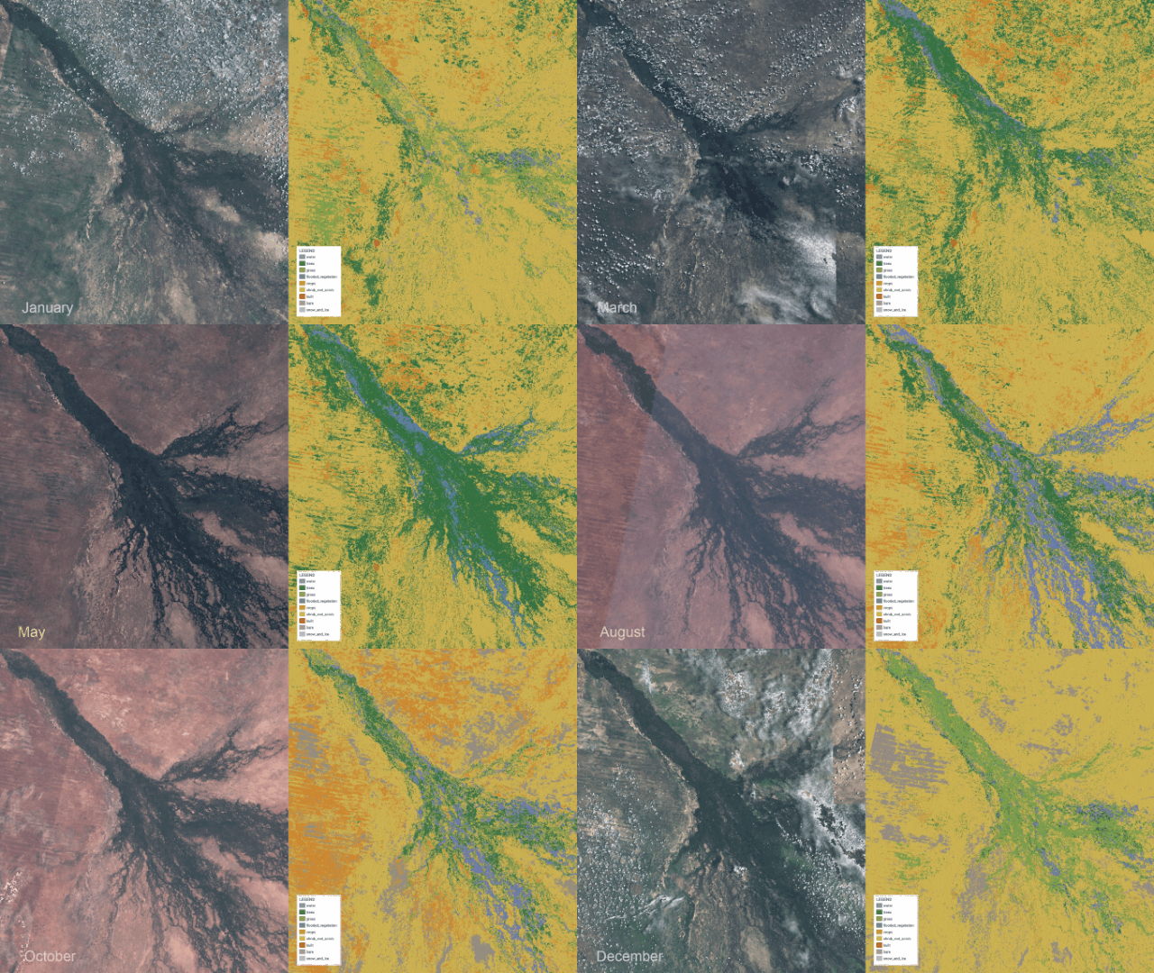
9个土地覆盖类别的每个像素

人工智能驱动方法的一个主要好处是该模型查看传入的Sentinel-2卫星图像，并且对于图像中的每个像素，估计树木覆盖程度、特定区域的建成情况或积雪覆盖。

10米分辨率

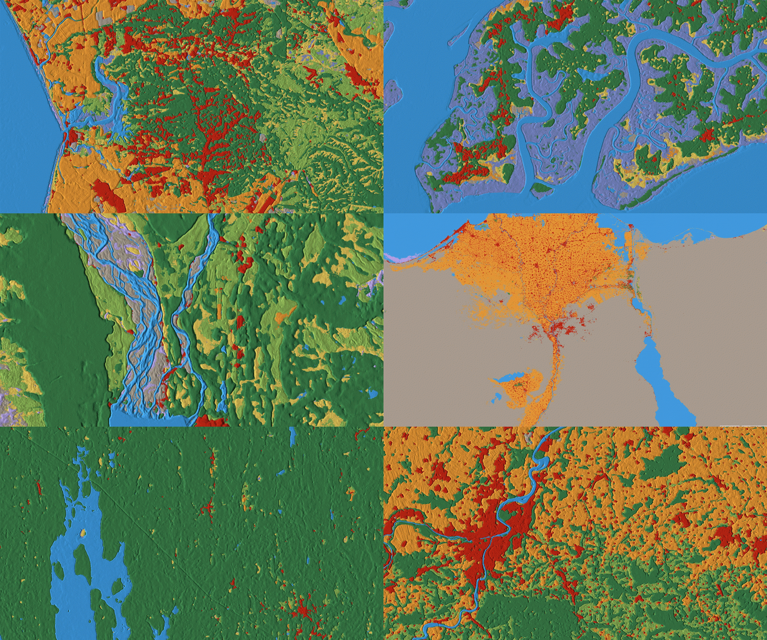
由于欧盟委员会的哥白尼计划使欧洲航天局哨兵数据免费和公开可用，Dynamic World等产品能够提供10m分辨率的土地覆盖数据，更高分辨率量化数据可以为地球表面的真实情况产生更准确的成果。

数据预览

Earth Engine Apps数据可视化（需要科学上网访问）：

https://sites.google.com/view/dynamic-world/home

https://www.dynamicworld.app/explore/

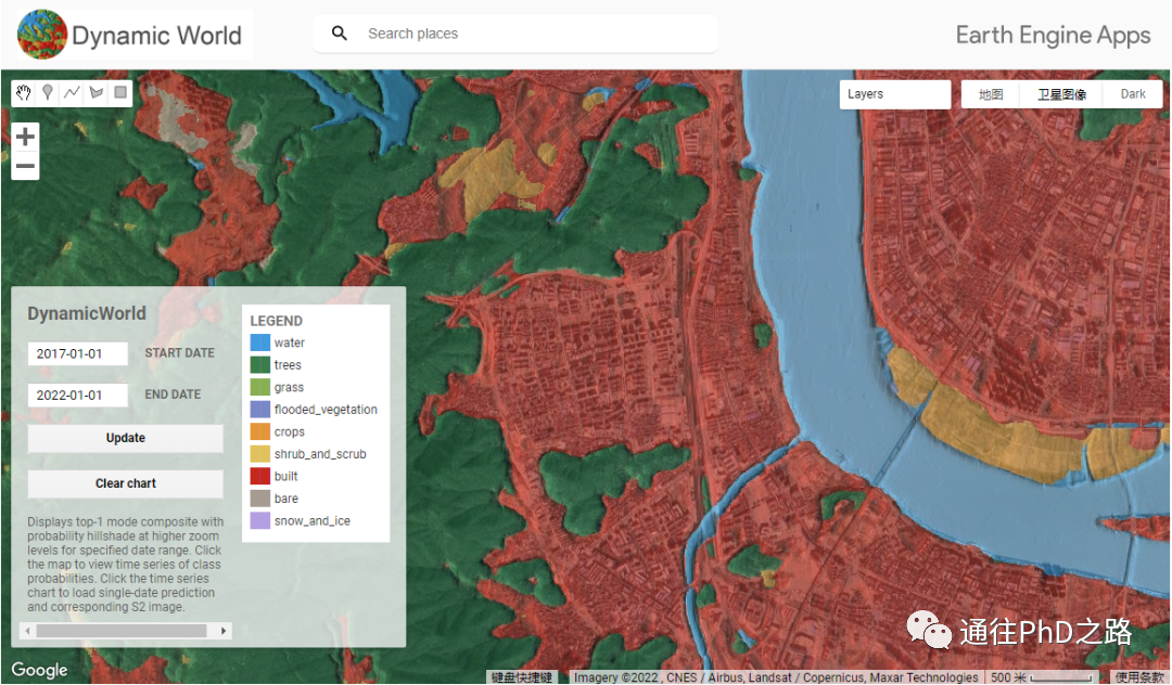
（可视化界面）

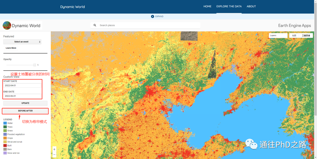
（设置时间和可视化模式，默认情况下是生成给定时间内的LUCC）

（切换为Before/After卷帘模式）

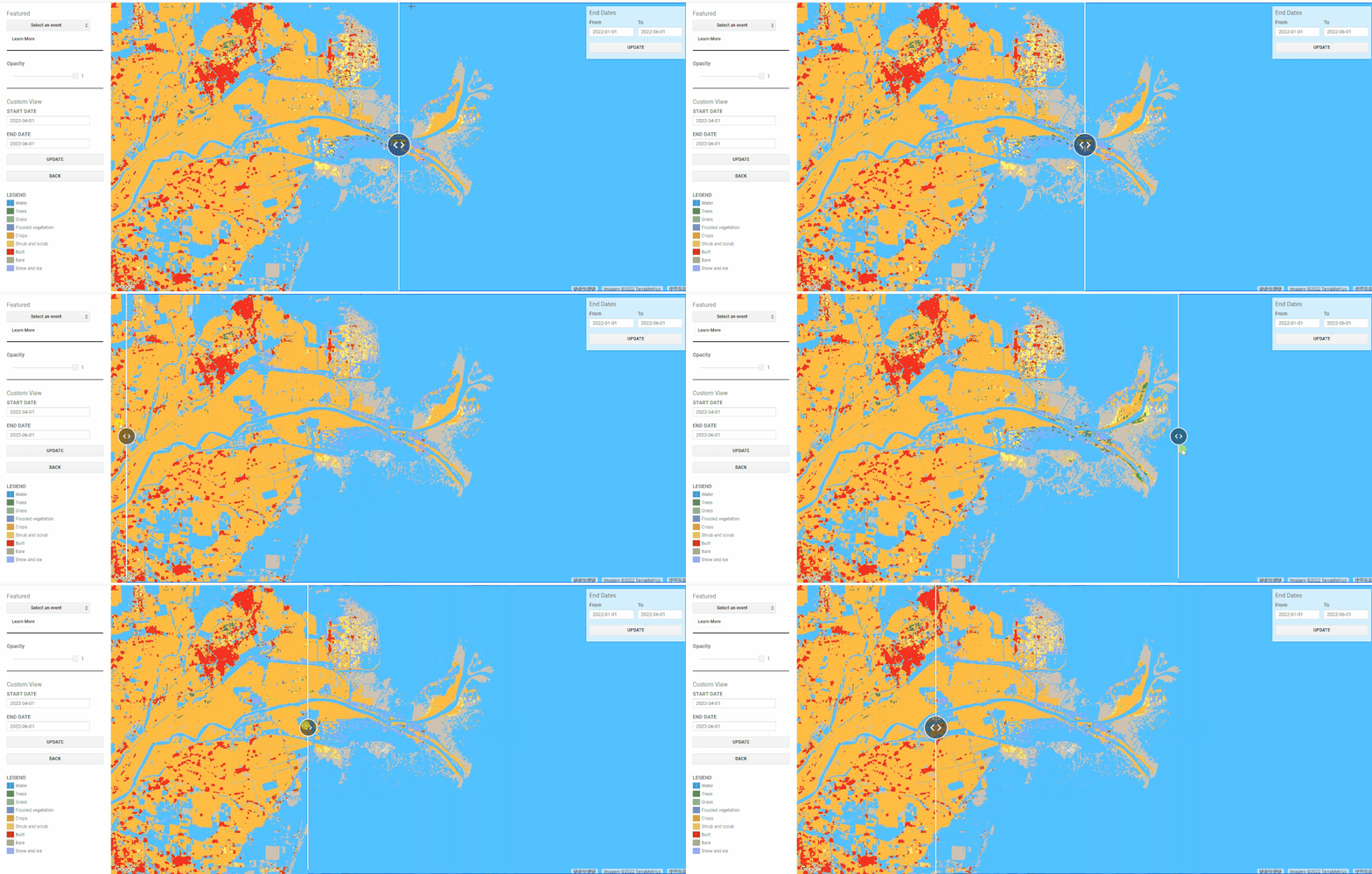
（黄河入海口2022-1-1与2022-6-1对比）

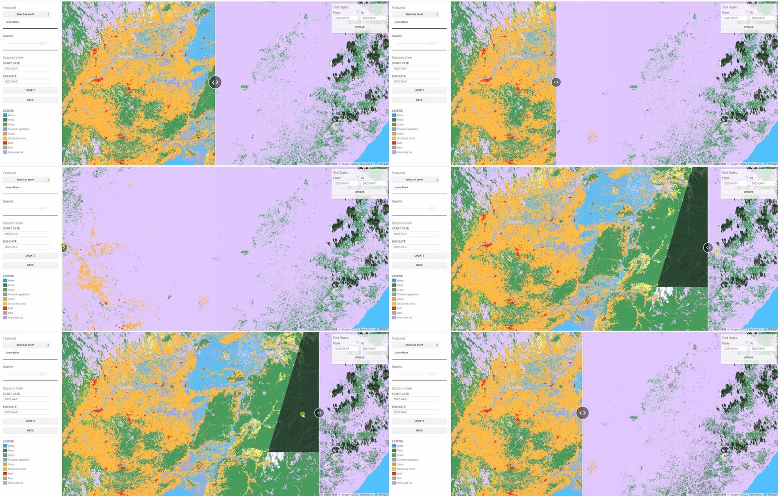
（东北三江平原2022-1-1与2022-6-1对比）

数据下载

该数据产品目前仅支持在GEE上使用。

网址：

https://developers.google.com/earth-engine/datasets/catalog/GOOGLE_DYNAMICWORLD_V1#bands (opens new window)

GEE仓库：

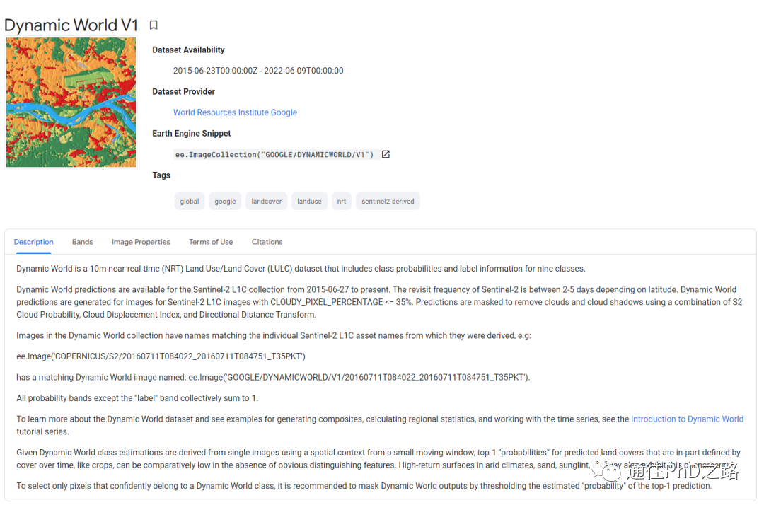
ee.ImageCollection("GOOGLE/DYNAMICWORLD/V1")

GEE代码:

链接：https://code.earthengine.google.com/234b0b83917e66e0f77b896ad731a283

代码:

//公众号  锐多宝的地理空间


// Creating Multi-Temporal Composites

// Extract the boundary for Dane County, Wisconsin
// from TIGER: US Countries 2018 dataset
var counties = ee.FeatureCollection('TIGER/2016/Counties');
var filtered = counties.filter(ee.Filter.eq('NAMELSAD', 'Dane County'));
var geometry = filtered.geometry();
Map.centerObject(geometry, 10)

// Filter the Dynamic World NRT collection
// for the year 2020 over the selected region.
var startDate = '2020-01-01';
var endDate = '2021-01-01';

var dw = ee.ImageCollection('GOOGLE/DYNAMICWORLD/V1')
  .filter(ee.Filter.date(startDate, endDate))
  .filter(ee.Filter.bounds(geometry))

// Create a Mode Composite
var classification = dw.select('label')
var dwComposite = classification.reduce(ee.Reducer.mode());

var dwVisParams = {
  min: 0,
  max: 8,
  palette: ['#419BDF', '#397D49', '#88B053', '#7A87C6',
    '#E49635', '#DFC35A', '#C4281B', '#A59B8F', '#B39FE1']
};

// Clip the composite and add it to the Map
Map.addLayer(dwComposite.clip(geometry), dwVisParams, 'Classified Composite') 

// Create a Top-1 Probability Hillshade Visualization
var probabilityBands = [
    'water', 'trees', 'grass', 'flooded_vegetation', 'crops',
    'shrub_and_scrub', 'built', 'bare', 'snow_and_ice'
    ];

// Select probability bands 
var probabilityCol = dw.select(probabilityBands)

// Create a multi-band image with the average pixel-wise probability 
// for each band across the time-period
var meanProbability = probabilityCol.reduce(ee.Reducer.mean())

// Composites have a default projection that is not suitable
// for hillshade computation.
// Set a EPSG:3857 projection with 10m scale
var projection = ee.Projection('EPSG:3857').atScale(10)
var meanProbability = meanProbability.setDefaultProjection(projection)

// Create the Top1 Probability Hillshade
var top1Probability = meanProbability.reduce(ee.Reducer.max())
var top1Confidence = top1Probability.multiply(100).int()
var hillshade = ee.Terrain.hillshade(top1Confidence).divide(255)
var rgbImage = dwComposite.visualize(dwVisParams).divide(255);
var probabilityHillshade = rgbImage.multiply(hillshade)

var hillshadeVisParams = {min:0, max:0.8}
Map.addLayer(probabilityHillshade.clip(geometry),
  hillshadeVisParams, 'Probability Hillshade')


// Export the Composite

// Raw Composite
Export.image.toDrive({
  image: dwComposite.clip(geometry),
  description: 'Raw_Composite_Export',
  fileNamePrefix: '2020_composite_raw',
  region: geometry,
  scale: 10,
  maxPixels: 1e10})

// Top1 Probability Hillshade Composite
var hillshadeComposite = probabilityHillshade.visualize(hillshadeVisParams)

Export.image.toDrive({
  image: hillshadeComposite.clip(geometry),
  description: 'Top1_Probability_Hillshade_Composite_Export',
  fileNamePrefix: '2020_composite_hillshade',
  region: geometry,
  scale: 10,
  maxPixels: 1e10})
  

（GEE数据目录及调用实例）

参考:Brown, C.F., Brumby, S.P., Guzder-Williams, B. et al. Dynamic World, Near real-time global 10 m land use land cover mapping. Sci Data 9, 251 (2022). https://doi.org/10.1038/s41597-022-01307-4.